Section 3. Aim of an atmospheric transport model in connection with numerical weather prediction (NWP) model (scientific information)
Aim of an atmospheric transport model in connection with numerical weather prediction (NWP) model (scientific information)
3.1 The portion of the atmosphere where the earth's surface (land or water) has a direct influence is called the Atmospheric Boundary Layer (ABL). Since most pollution releases occur in that layer, (except for aircraft emissions, volcanic eruptions or high level bomb blasts) it is important to review some fundamental concepts about the ABL structure.
3.1.1 The main feature of the Atmospheric Boundary Layer is the turbulent nature of the flow. Turbulence reinforces mixing mechanisms and tends to homogenize the properties of the atmospheric fluid much more quickly than would a laminar flow. For example turbulent mixing is an important factor in preventing local accumulation of anthropogenic pollutants.
3.1.2 The meteorological parameters are affected by the earth's surface through dynamical processes (friction of the air over the surface) and through thermal processes (heating or cooling of the air in contact with the ground).
At the top of the ABL, in the free atmosphere, the wind speed is approximately geostrophic. At the surface, the wind speed reduces to zero over land, and matches the speed of the surface currants over water. Hence a wind shear exits over the depth of the ABL which dynamically produces turbulence. The stronger is the wind aloft, the more intense is the generated turbulence. This mechanical turbulence produces a flux of momentum from the atmosphere to the surface of the earth. When there is a difference between the temperature of the surface and the temperature of the air, there is a transfer of energy between the two bodies, and a heat flux is created within the ABL. These fluxes are very different, depending on the vertical temperature gradient. Close to the surface, there exists a layer were the fluxes of heat and momentum are nearly constant with height; this layer is called the surface boundary layer (SBL) or more simply, the surface layer. In that layer, frictional effects are dominant compared to pressure and Coriolis forces. The scaling length is zo, the roughness length, which is the height above the ground where the wind is assumed to vanish in order to take into account the rough elements of the surface. Generally three states of ABL are distinguished : neutral, unstable and stable.
3.1.3 In the neutral ABL, the temperature of the surface is equal to the temperature of the air. A truly neutral ABL (potential temperature uniform throughout the whole ABL, only mechanical turbulence) is infrequent. Within the SBL the vertical wind follows a logarithmic profile. Above the SBL, the Coriolis force becomes important and the wind turns (clockwise in the Northern Hemisphere and anticlockwise in the Southern Hemisphere) with the altitude. The wind increases with height to become equal to the geostrophic wind in the free atmosphere, both in direction and velocity, at the top of the ABL.
3.1.4 In the unstable ABL, the temperature of the surface is greater than the temperature of the air (the surface heats the air). Buoyancy forces compound the mechanical effects and intense turbulence is generated. This layer can be divided into three zones: first, the surface layer (typically tens of meters) with an superadiabatic gradient of temperature and a rather strong wind shear, second, a mixed layer where the potential temperature and winds are almost constant with height, and third, an entrainment zone where there is a temperature inversion which caps the ABL. In the capping inversion zone, the turbulence is damped by a strong stable stratification. Some coherent structures can be frequently identified within the unstable ABL, such as convective cells or warm parcels, and can be studied as a separate subject. The unstable ABL occurs generally during the day when the solar heating is important.
3.1.5 In the stable ABL, the temperature of the surface is lower than the temperature of the air (the air heats the surface). The thermal effects in that case counteract the motions induced by mechanical turbulence. The surface layer shows an subadiabatic gradient of temperature over a depth of roughly ten meters. Pollutants released in that layer remain near the source. The wind is generally weak near the surface and a maximum (low level jet) is often found at the top of the temperature inversion zone. The stable ABL usually occurs during the night. In those conditions, the stable ABL is capped by an unstable layer, remnant of the ABL produced during the previous day and in which only the dynamical turbulence remains.
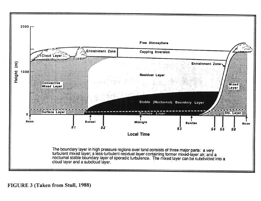
3.1.6 Generally the definition of the height of the ABL is rather arbitrary. For example, the height of the ABL can be identified as the altitude where the mean vertical turbulent fluxes becomes "negligible". Fortunately, the ABL is often capped with a temperature inversion zone; in that case h is equal to zi, the altitude of the bottom of this capping inversion layer. The typical height of the ABL is about 1500 meters. The diurnal variation of the ABL is illustrated in figure 3 ( Stull, 1988).
3.1.7 Many theoretical studies of the ABL have been done. The Ekman model (1902) is interesting because it provides a simple estimate of the wind variation over the whole ABL. Ekman assumed a three-way balance among the Coriolis force, the pressure gradient force and the frictional forces due to turbulent motion. It was further assumed, that these frictional forces were proportional to the vertical shear of the mean horizontal wind, that the proportionality factor (the eddy diffusivity coefficient) was constant, and that the pressure gradient forces were constant in the ABL (i.e. constant geostrophic wind). With these assumptions the equations of motion lead the well known Ekman wind spiral (see Appendix 1, referenced below). It predicts an angle of 45N between the surface wind and the geostrophic wind. Typically, the observed angle is about 10N in unstable conditions, 15 to 20N in neutral conditions, and 30 to 50N in stable conditions. It is in the stable ABL that the Ekman model applies best.
3.1.8 A widely accepted model to describe the surface layer is provided by the Similarity Theory which states that the mean and turbulent properties in the layer depend only on the height z, and three governing parameters: a buoyancy parameter, the surface wind stress and the surface heat flux. These three governing parameters define a length scale, the Monin-Obukhov length L, a velocity scale u*, and a temperature scale q*. Wind and temperature profiles are given as universal functions of dimensionless combination of these scaling parameters together with the roughness parameter z0 (see Appendix 2 for more details, referenced below).
3.2 With these basic principles, it is now possible to consider the modelling of the transport and diffusion of a pollutant in the atmosphere. All ATMs are governed by the "advection-diffusion equation", which is the equation of continuity for the concentration of pollutant C .
3.2.1 The advection-diffusion equation states that the time variation of the concentration of pollutant at a point depends on several different physical processes (see Appendix 3, referenced below). These processes are:
a) advection or transport by the mean wind.b) diffusion or mixing by unresolved turbulent wind eddies; in reality it is also a transport process occurring at scales which cannot be fully resolved and which must be parameterized in some fashion. The combined processes of advection and diffusion are often commonly referred to as dispersion.
c) emission describing the processes by which pollutants are released in the atmosphere.
d) depletion describing the processes by which pollutants are removed from the atmosphere. These generally take into account the effects of clouds and precipitation (wet scavenging), radioactive decay, and deposition on the ground due to the various capturing properties of the surface (dry deposition).
3.2.2 There are several types of models to simulate the Long Range Transport and Diffusion of pollutants in the atmosphere: they mainly fall in two classes Lagrangian ATMs and the Eulerian ATMs.
Lagrangian models describe fluid elements that follow the instantaneous wind flow. They include all models in which plumes can be broken down into segments, puffs or particles. The advection is directly simulated by computing the trajectories of the plume elements as they move in the mean wind field. In models where the plume is modelled by a relatively low number of elements (puffs or plume segments) diffusion is usually simulated by a Gaussian model applied to each plume elements, and where the standard deviation is calculated taking into account the ABL structure. Some ATMs use a very large number of particles and diffusion is modelled by adding a "semi-random" component to the large scale wind, using Monte Carlo techniques. The probability density function for the random component, which simulates the atmospheric turbulence, is also dependent on the state of the ABL. The trajectory of each particles is calculated using these pseudovelocities, and concentrations are calculated by counting the number of particles within a certain volume.
Eulerian models directly solve the diffusion equation at every point of a grid, using numerical techniques that allow specific treatments for each physical process (finite difference method, splitting, finite elements method ...). The turbulent fluxes are commonly assumed to be proportional to the mean gradient according to the K gradient theory (first order closure). The horizontal and vertical K coefficients are generally dependent on the ABL structure. Precautions have to be taken in order to minimize the artificial diffusion frequently introduced by the numerical approximations.
3.3 The modelling of the source of emission, the source term description, is a crucial part of ATMs. In most cases, the processes by which pollutants are injected in the atmosphere (explosion, fire, high pressure jet, etc.) happen at scales well below those which are resolved by ATMs. The source effects have to be parameterized; the type of parameterization will depend on whether the ATM is Lagrangian or Eulerian.
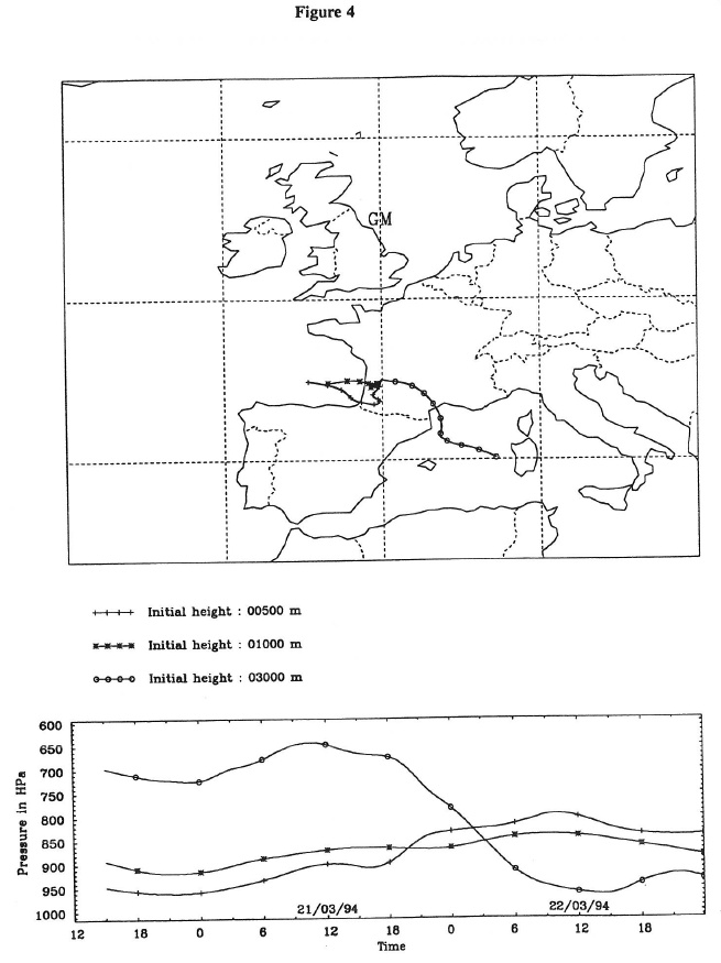
3.3.1 Information on the initial release height and its vertical extent is essential. This is illustrated in figure 4, which shows three trajectories starting at the same time but at different heights. Two of them are in the ABL (500 m and 1000 m), the third one is in the free atmosphere. The results are very different, even for the "in ABL" trajectories. In this extreme case, a release in the lower layer (< 500m) would have moved south then westward along the France-Spain border towards the Atlantic ocean. A release around 1000m would have gone straight West over the Atlantic. In the in the free atmosphere, however, a release would have moved eastward at the beginning, then southward over the Mediterranean sea. Deciding on the proper countermeasures in this particular situation would not have been very easy, if no estimate of the vertical extension of the release would have been available.
3.3.2 The time scenario is also of major importance. Of course the state of the atmosphere changes considerably with time: frontal passages, movement of pressure systems, diurnal evolution of the ABL, etc.. These will profoundly affect the evolution of the pollution cloud. For example, if a front moves over the source area, wet deposition could be a major factor for ground contamination; the deposition areas would be completely different if the release had begun before or after the arrival of the front. Furthermore, the transport/diffusion processes would also be very different and the pollutant plumes would reach different regions.
3.3.3 If the vertical structure and the time scenario of the source term are well described, a rough estimate of the amount of pollutant is generally enough to decide on suitable countermeasures: protection of the population, food restriction, etc.. In certain cases, the area of maximum air concentration and the deposition areas need only to be qualitatively known, and more accurate estimation of the plume intensity would come out of ground measurements. If accurate estimates of the amount of pollutant released are available (which seems unlikely in a emergency), the ATM could yield outputs of qualitative and quantitative interest.
3.3.4 Information on the radiological species released is important because parameters such as dry deposition velocity, scavenging ratio, and half life are dependent on the type of pollutant; all of the depletion terms of the diffusion equation are directly related to the nature of the released elements.
3.4 Generally, ATMs used during emergencies are diagnostic or "off side" models, in order to allow for a fast and timely response. The dispersion calculations are not performed within a full scale NWP; rather, the ATMs are stand-alone models which must be provided with meteorological data from NWP models as input. So there is an impact of NWP models on the ATMs. NWP models provide data on a grid with a specific scale and all the information produced by NWP models is not necessarily available. ATMs can only simulate phenomena of the same scale as the input data mesh and sub-grid scale phenomena have to be parametrized. That is the main reason why processes such as convection or scavenging are treated in a cruder fashion in operational ATMs than in research ATMs. ATMs are of course dependent on the quality of the input meteorological data. A source of uncertainty is the precipitation field. NWP models generally only provide rain fluxes at the ground, so estimation of the depth of the wet layer must be done by ATMs. The results for wet deposition may not be very accurate, even when the precipitation areas are well estimated. ATMs will reproduce, and sometimes amplify, the NWP models errors. In the ATMES (Klug et al., 1992) experiment, evaluation of different ATMs for the Chernobyl accident, has shown that the evolution of a pollution cloud can be depicted fairly well when analysed/observed meteorological fields are used. However there is a deterioration of the models' performance when using forecast meteorological fields. That is why an evaluation of the NWP forecasts by senior meteorologists is essential. Experienced forecasters can advise the ATM specialists about the quality of the forecast meteorological fields so that the quality of the outputs of ATMs can be assessed.
3.5 ATMs can provide a large variety of calculations and ouptuts. However in the case of the basic standard products produced by the RSMCs, there are three kinds of outputs: time-integrated air concentrations of pollutant in Becquerel second per cubic metre, the total (dry and wet) cumulated deposition at the ground in Becquerel per square metre and air trajectories starting at three standard levels.
3.5.1 The time-integrated air output is obtained by computing the mean air concentration over the 500 first meters at each time step, and then integrating it over a predefined period. The results can then be used to calculated doses received by a human being who would remain at a given location during the considered period.
3.5.2 The total cumulated deposition represents, for a radiological pollutant, the activity which is present at the surface after a certain duration followin the start of the release. On this chart, dry deposition due to the uptake of pollutant by the ground and wet deposition due to precipitation are added. It represents the impact at the ground for the radiological event.
3.5.3 The air trajectories represent the motion of an air parcel within the three dimensional wind field. These trajectories can reveal interesting information about the vertical structure of the atmosphere and the differences in the flow as a function of height in the vicinity of the source of emission. It can also help explain to some degree the dispersing plume shapes. Trajectories can also provide information about differences in the predicted wind fields from different meteorological models.
Appendix 1: The Ekman wind spiral
Appendix 2: The Surface Boundary Layer and the Similarity Theory
Appendix 3: The advection diffusion equation
REFERENCES
STULL, R.B., 1988. An Introduction to Boundary Layer Meteorology. Kluwer Academic Publishers, Boston.
KLUG W., Graziani G., Gripa G., Pierce D and C. Tassone, 1992. Evaluation of Long Range Atmospheric Transport Models Using Environmental Radioactivity Data From The Chernobyl Accident: The ATMES Report. Elsevier Science Publishers Ltd., London and New York.
Updated 6 May 2014