The State of Greenhouse Gases in the Atmosphere Using Global Observations through 2012
Supplementary materials to the WMO Greenhouse Gas Bulletin N.9
Executive summary
The latest analysis of observations from the WMO Global Atmosphere Watch (GAW) Programme shows that the globally averaged mole fractions of carbon dioxide (CO2), methane (CH4) and nitrous oxide (N2O) reached new highs in 2012, with CO2 at 393.1±0.1 ppm[2], CH4 at 1819±1 ppb[3] and N2O at 325.1±0.1 ppb. These values constitute, respectively, 141%, 260% and 120% of pre-industrial (before 1750) levels. The atmospheric increase of CO2 from 2011 to 2012 is higher than the average growth rate over the past 10 years. For N2O the increase from 2011 to 2012 is smaller than the one observed from 2010 to 2011 but larger than the average growth rate over the past 10 years. Atmospheric CH4 continued to increase at a rate similar to the one observed over the past 4 years. The National Oceanic and Atmospheric Administration (NOAA) Annual Greenhouse Gas Index shows that from 1990 to 2012 radiative forcing by long-lived greenhouse gases increased by 32%, with CO2 accounting for about 80% of this increase. |
Overview
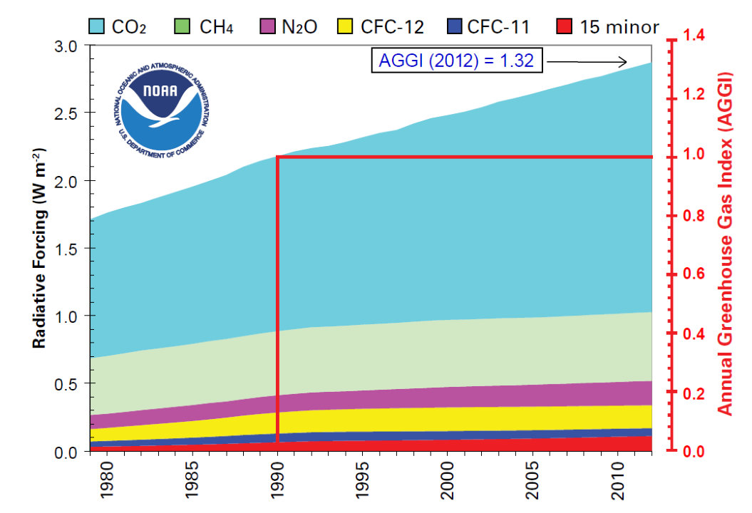
This ninth WMO/GAW Annual GHG Bulletin reports atmospheric abundances and rates of change of the most important long-lived greenhouse gases (LLGHGs) – carbon dioxide, methane, nitrous oxide – and provides a summary of the contributions of the other gases. These three together with CFC-12 and CFC-11 account for approximately 96%[4] of radiative forcing due to LLGHGs (Figure 1).
Figure 1. Atmospheric radiative forcing, relative to 1750, of LLGHGs and the 2012 update of the NOAA Annual Greenhouse Gas Index (AGGI). |
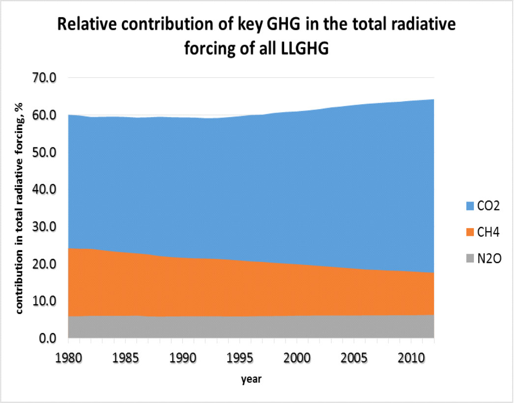
Figure 1 (additional). Changing contribution (in %) of key greenhouse gases in the total radiative forcing of all LLGHG. |
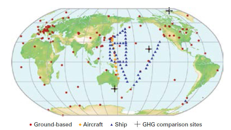
The WMO Global Atmosphere Watch Programme (http://www.wmo.int/gaw) coordinates systematic observations and analysis of greenhouse gases and other trace species. Sites where greenhouse gases are monitored in the last decade are shown in Figure 2. During 2012, the number of observational stations declined. Measurement data are reported by participating countries and archived and distributed by the World Data Centre for Greenhouse Gases (WDCGG) at the Japan Meteorological Agency.
Number of stations used for the calculation of the global averages.
CO2 |
121 |
CH4 |
120 |
N2O |
28 |
SF6 |
20 |
CFC-11 |
19 |
CFC-12 |
19 |
CFC-113 |
19 |
CCl4 |
15 |
CH3CCl3 |
18 |
HCFC-141B |
8 |
HCFC-142B |
12 |
HCFC-22 |
12 |
HFC-134A |
8 |
HFC-152A |
7 |
|
Figure 2. The GAW global network for carbon dioxide in the last decade. The network for methane is similar.
Table 1 provides globally averaged atmospheric abundances of the three major LLGHGs in 2012 and changes in their abundances since 2011 and 1750. The results are obtained from an analysis of datasets (WMO, 2009) that are traceable to WMO World Reference Standards. Data from mobile stations, with the exception of NOAA sampling in the Pacific (blue triangles in Figure 2), are not used for this global analysis.
|
Table 1. Global annual mean abundances (2012) and trends of key greenhouse gases from the WMO/GAW global greenhouse gas monitoring network. Units are dry-air mole fraction, and uncertainties are 68% confidence limits.
|
CO2 |
CH4 |
N2O |
Global abundance in 2012 |
393.1±0.1[5] ppm |
1819±1[5] ppb |
325.1±0.1[5] ppb |
2012 abundance relative to year 1750* |
141% |
260% |
120% |
2011-12 absolute increase |
2.2 ppm |
6 ppb |
0.9 ppb |
2011-12 relative increase |
0.56 % |
0.33 % |
0.28 % |
Mean annual absolute increase during last 10 years |
2.02 ppm/yr |
3.7 ppb/yr |
0.80 ppb/yr |
* Assuming a pre-industrial mole fraction of 278 ppm for CO2, 700 ppb for CH4 and 270 ppb for N2O.
The three greenhouse gases shown in the Table 1 are closely linked to anthropogenic activities and they also interact strongly with the biosphere and the oceans. Predicting the evolution of the atmospheric content of greenhouse gases requires an understanding of their many sources, sinks and chemical transformations in the atmosphere.
The NOAA Annual Greenhouse Gas Index (AGGI) in 2012 was 1.32, representing a 32% increase in total radiative forcing (relative to 1750) by all LLGHGs since 1990 and a 1.2% increase from 2011 to 2012 (Figure 1). The total radiative forcing by all LLGHGs in 2012 corresponds to a CO2-equivalent mole fraction of 475.6 ppm (http://www.esrl.noaa.gov/gmd/aggi).
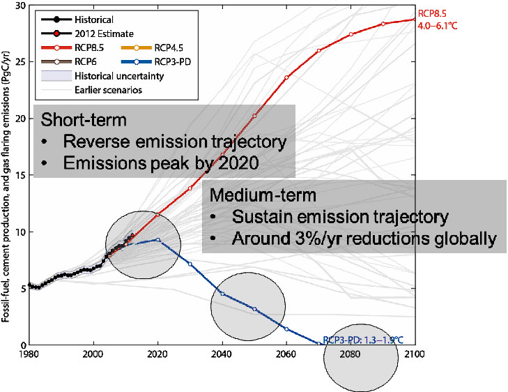
Implications for climate: Challenges to keep below 2ºC
Source: Peters et al. 2013; Global Carbon Project 2012 |
|
|
An emission pathway with a “likely chance” to keep the temperature increase below 2ºC has significant challenges |
Role of the greenhouse gases in total radiative forcing (Working Group I Contribution to the IPCC Fifth Assessment Report Climate Change 2013: The Physical Science Basis, Figure SPM.5)
|
|
Carbon Dioxide (CO2)
Carbon dioxide is the single most important anthropogenic greenhouse gas in the atmosphere, contributing ~64%[4] to radiative forcing by LLGHGs. It is responsible for ~84% of the increase in radiative forcing over the past decade and ~82% over the past five years. The pre-industrial level of ~278 ppm represented a balance of fluxes between the atmosphere, the oceans and the biosphere.
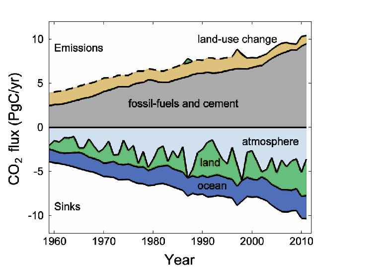
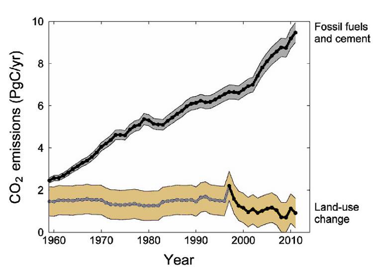
Global Carbon Emisisons and Budget
Source: Le Quéré et al. 2012; Global Carbon Project 2012 |
The dashed land-use change line does not include management-climate interactions.
The land sink was a source in 1987 and 1998 (1997 visible as an emission). |
Total global emissions in 2011 are 37% over 1990.
Percentage land-use change: 36% in 1960, 18% in 1990, 9% in 2011. Land-use change black line: Includes management-climate interactions. |
|
Atmospheric CO2 reached 141% of the pre-industrial level in 2012, primarily because of emissions from combustion of fossil fuels (fossil fuel CO2 emissions 9.5±0.5 PgC[1] in 2011 according to http://www.globalcarbonproject.org), deforestation and other land-use change (0.9±0.5 PgC[1] in 2011). The average increase in atmospheric CO2 from pre-industrial time corresponds to ~55% of the CO2 emitted by fossil fuel combustion with the remaining ~45% removed by the oceans and the terrestrial biosphere. The portion of CO2 emitted by fossil fuel combustion that remains in the atmosphere (airborne fraction), varies interannually due to high natural variability of CO2 sinks (Levin, 2012) without a confirmed global trend.
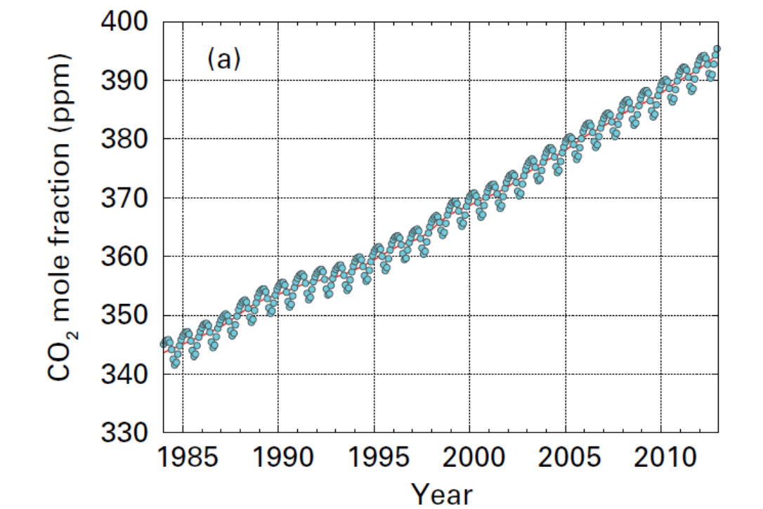
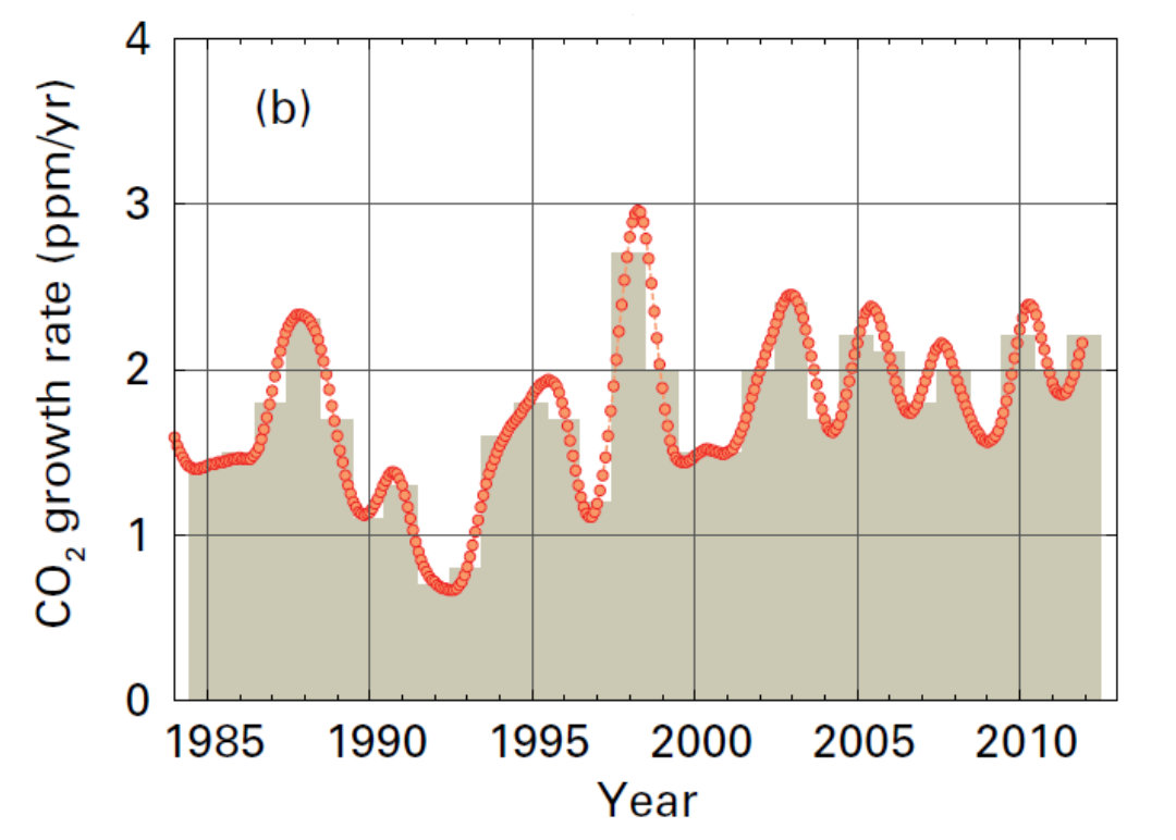
The globally averaged CO2 mole fraction in 2012 was 393.1±0.1 ppm (Figure 3). The increase in annual mean since 2011, 2.2 ppm, is greater than the increase from 2010 to 2011, the average growth rate for the 1990s (~1.5 ppm/yr) and the average growth rate for the past decade (~2.0 ppm/yr).
Monthly means of CO2 mixing ratios up to 2011 are shown on the plot (Figure 3add, click to enlarge). The graph shows a substantial increase of the mixing ratio at all reporting stations and exceedances of the “symbolic” values of 400ppm at a number of stations in the Northern Hemisphere. |
Figure 3 (additional): Monthly mean CO2 mole fractions that have been reported to the WDCGG. The sites are listed in order from north to south (from WDCGG Data Summary No.37)
|
|
|
Figure 3. Globally averaged CO2 mole fraction (a) and its growth rate (b) from 1984 to 2012. Annually averaged growth rates are shown as columns in (b). |
Importance of the CO2 sinks: Cover story of the GHG Bulletin No.8 (2012)
The “other” CO2 problem – Ocean acidification
Profound changes in seawater chemistry are underway as the ocean takes up about one fourth of the anthropogenic CO2 emitted to the atmosphere year-on-year. This phenomenon, known as ocean acidification, has emerged as a key issue of global concern in the last fifteen years. Some facts about ocean acidifications can be found in “20 Facts about ocean acidification”.The Ocean Acidification International Coordination Centre (OA-ICC) works to promote, facilitate and communicate global activities on ocean acidification.
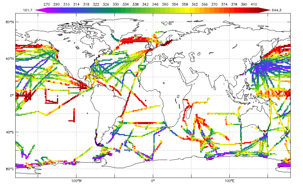
At the “Surface Ocean CO2 Variability and Vulnerability” (SOCOVV) workshop at UNESCO, Paris in April 2007, participants agreed to establish a global surface CO2 data set that would bring together, in a common format, all publicly available fCO2 data for the surface oceans. This work allowed to map the distribution of fCO2 in Surface Ocean CO2 Atlas (SOCAT, www.socat.info/about.html), which includes:
| - a 2nd level quality controlled global surface ocean fCO2 data set following agreed procedures and regional review,
- and a gridded SOCAT product of monthly surface water fCO2 means on a 1° x 1° grid with no temporal or spatial interpolation.
|
EXAMPLE: SOCAT product for January
|
|
Methane (CH4)
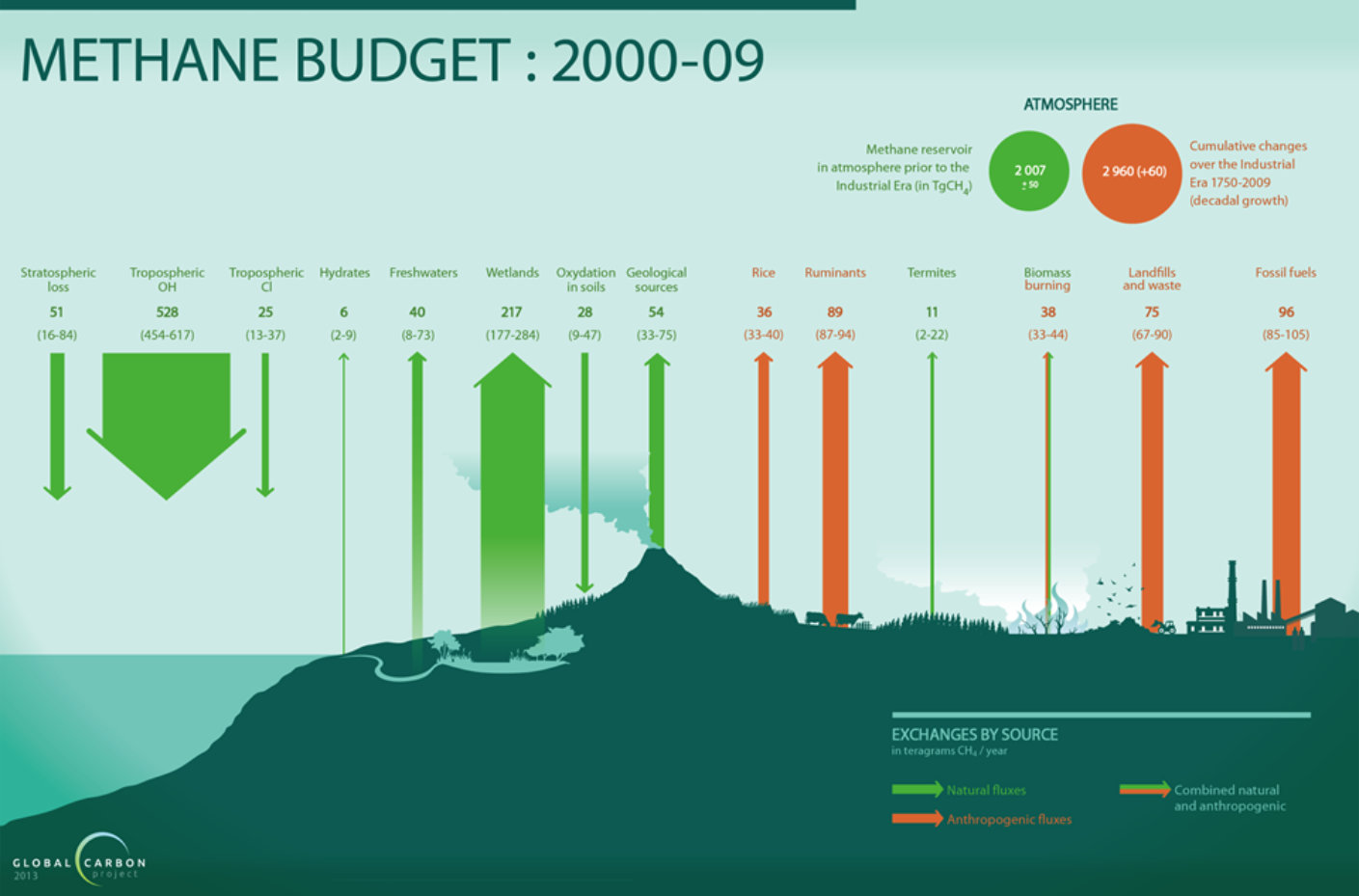
Methane contributes ~18%[4] to radiative forcing by LLGHGs. Approximately 40% of methane is emitted into the atmosphere by natural sources (e.g., wetlands and termites), and about 60% comes from anthropogenic sources (e.g., ruminants, rice agriculture, fossil fuel exploitation, landfills and biomass burning).
(Global Carbon Project 2013; Figure based on Kirschke et al. 2013, Nature Geoscience)
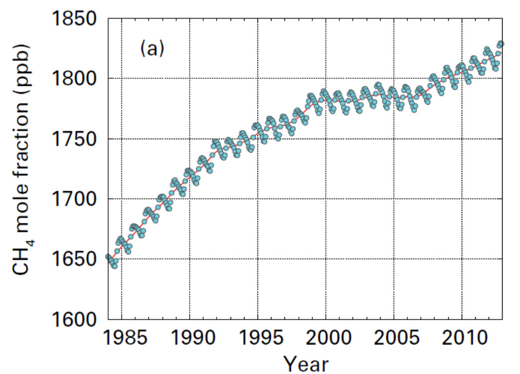
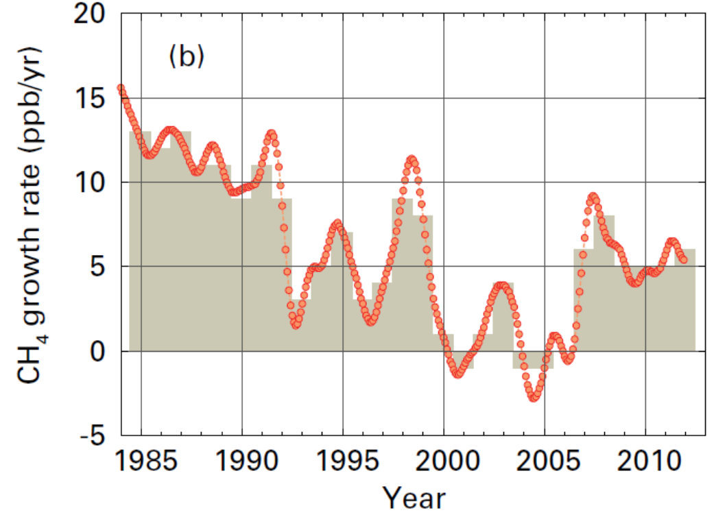
Atmospheric CH4 reached 260% of the pre-industrial level (~700 ppb) due to increased emissions from anthropogenic sources. Globally averaged CH4 reached a new high of 1819 ± 1 ppb in 2012, an increase of 6 ppb with respect to the previous year (Figure 4). The growth rate of CH4 decreased from ~13 ppb/yr during the early 1980s to near zero during 1999-2006. Since 2007, atmospheric CH4 has been increasing again due to increased emissions in the tropical and mid-latitude Northern Hemisphere. The attribution of this increase to anthropogenic and natural sources is difficult because the current network is insufficient to characterize emissions by region and source process.
Figure 4 (additional 1): Monthly mean CH4 mole fractions that have been reported to the WDCGGup to the end on 2011. The sites are listed in order from north to south (from WDCGG Data Summary No.37). |
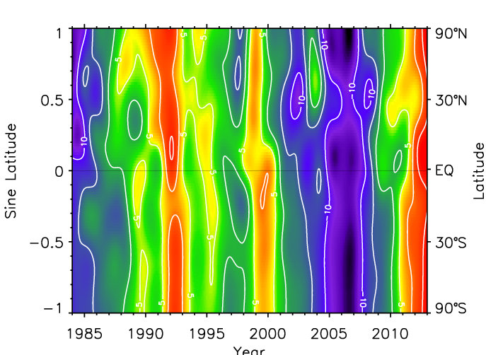
Figure 4 (additional 2): Anomaly of methane monthly mean mole fraction distribution. Strong positive anomalies were observed in polar latitudes in 2007. (The plot is a courtesy of Ed Dlugokencky, NOAA).
|
|
|
| Figure 4. Globally averaged CH4 mole fraction (a) and its growth rate (b) from 1984 to 2012. Annually averaged growth rates are shown as columns in (b). |
Attribution of methane abundance changes: cover story of this Bulletin.
Nitrous Oxide (N2O)
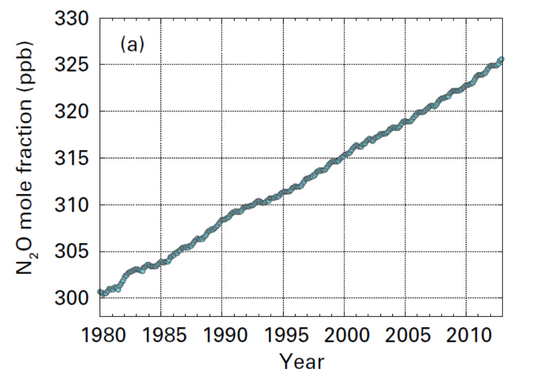
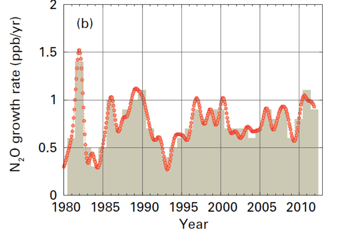
Nitrous oxide contributes ~6%[4] to radiative forcing by LLGHGs. It is the third most important contributor to the combined forcing. N2O is emitted into the atmosphere from both natural (about 60%) and anthropogenic sources (approximately 40%), including oceans, soil, biomass burning, fertilizer use, and various industrial processes. The globally averaged N2O mole fraction in 2012 reached 325.1 ±0.1 ppb, which is 0.9 ppb above the previous year (Figure 5) and 120% of the pre-industrial level (270 ppb). The annual increase from 2011 to 2012 is greater than the mean growth rate over the past 10 years (0.80 ppb/yr). |
Figure 5 (additional): Monthly mean N2O mole fractions that have been reported to the WDCGG. The sites are listed in order from north to south (from WDCGG Data Summary No. 37). |
|
|
|
| Figure 5. Globally averaged N2O mole fraction (a) and its growth rate (b) from 1980 to 2012. Annually averaged growth rates are shown as columns in (b). |
Other greenhouse gases
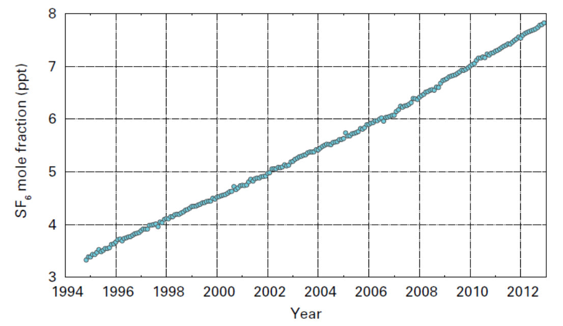
| Sulfur hexafluoride (SF6) is a potent LLGHG. It is produced by the chemical industry, mainly as an electrical insulator in power distribution equipment. Its current mole fraction is about twice the level observed in the mid-1990s (Figure 6). |
Figure 6. Monthly mean mole fraction of sulfur hexafluoride (SF6) from 1995 to 2012 (based on the measurements at 20 stations).
|
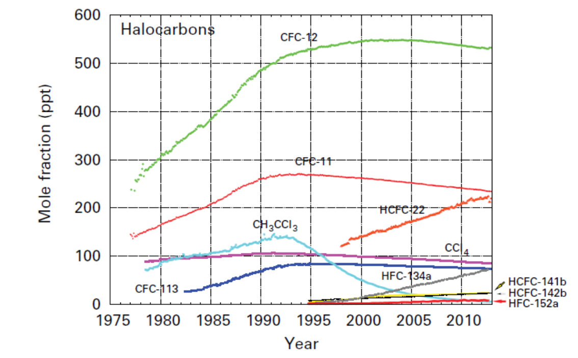
| The stratospheric-ozone- depleting chlorofluorocarbons (CFCs), together with minor halogenated gases, contribute ~12%[4] to radiative forcing by LLGHGs. While CFCs and most halons are decreasing, hydrochlorofluorocarbons (HCFCs) and hydrofluorocarbons (HFCs), which are also potent greenhouse gases, are increasing at relatively rapid rates, although they are still low in abundance (at ppt[6] levels, Figure 7). |
Figure 7. Monthly mean mole fractions of the most important halocarbons from 1977 to 2012 averaged over the network (based on the measurements between 7 and 19 stations).
|
This bulletin primarily addresses LLGHGs. Relatively short-lived tropospheric ozone has a radiative forcing comparable to that of the halocarbons. Many other pollutants, such as carbon monoxide, nitrogen oxides and volatile organic compounds, although not referred to as greenhouse gases, have small direct or indirect effects on radiative forcing. Aerosols (suspended particulate matter), too, are short-lived substances that alter the radiation budget. All gases mentioned herein, as well as aerosols, are monitored by the GAW Programme, with support from WMO Member countries and contributing networks.
Acknowledgements and links
Fifty WMO member countries have contributed CO2 data to the GAW WDCGG. Approximately 47% of the measurement records submitted to WDCGG are obtained at sites of the NOAA ESRL cooperative air-sampling network. For other networks and stations see GAW Report No. 206 (available at http://www.wmo.int/gaw). The Advanced Global Atmospheric Gases Experiment (AGAGE) is contributing observations to this bulletin. Furthermore, the GAW monitoring stations contributing data to this bulletin, shown in Figure 2, are included in the list of contributors on the WDCGG web page (http://ds.data.jma.go.jp/gmd/wdcgg/). They are also described in the GAW Station Information System, GAWSIS (http://gaw.empa.ch/gawsis) supported by MeteoSwiss, Switzerland.
References
Bergamaschi, P., Houweling,S., Segers, A., et al.: Atmospheric CH4 in the first decade of the 21st century: Inverse modeling analysis using SCIAMACHY satellite retrievals and NOAA surface measurements, J. Geophys. Res., 118, 7350–7369, 2013, doi:10.1002/jgrd.50480
Conway, T. J., Tans, P. P. , Waterman, L. S., Thoning, K. W., Kitzis, D. R., Masarie, K. A. and Zhang, N. Evidence for interannual variability of the carbon cycle from the National Oceanic and Atmospheric Administration/Climate Monitoring and Diagnostics Laboratory global air sampling network, J. Geophys. Res., 99, 22831-22855, 1994.
Levin, I., Earth science: The balance of the carbon budget, Nature, 488, 35–36, 2012, doi:10.1038/488035a
WMO, 2009: Technical Report of Global Analysis Method for Major Greenhouse Gases by the World Data Centre for Greenhouse Gases (Y. Tsutsumi, K. Mori, T. Hirahara, M. Ikegami and T.J. Conway). GAW Report No. 184 (WMO/TD No. 1473), Geneva, 29 pp.
Notes:
Terms used in this Bulletin are explained in the glossary.
|